APERTURE AND TOLERANCES

EUROPEAN ORGANIZATION FOR NUCLEAR RESEARCH

Defining aperture in MAD-X

A new feature of MAD-X is the ability to set an aperture for a particular element, or parent of a set of elements. This removes the need of placing a collimator next to every element to do aperture tracking. The aperture of any elements can be specified (excepts drifts) by the use of the following parameters:

APERTYPE This can have seven text values: CIRCLE, RECTANGLE, ELLIPSE, LHCSCREEN (a superposition of a CIRCLE and a RECTANGLE), MARGUERITE (two LHCSCREENS, one rotated by 90 degrees), RECTELLIPSE (a superposition of an ELLIPSE and a RECTANGLE) and RACETRACK.

APERTURE This is an array of values, the number and meaning of which depends on the APERTYPE:

APERTYPE	# of parameters	meaning of parameters
CIRCLE	1	radius
ELLIPSE	2	horizontal half axis, vertical half axis
RECTANGLE	2	half width and half height
LHCSCREEN	3	half width, half height (of rect.) and radius (of circ.)
MARGUERITE	3	half width, half height (of rect.) and radius (of circ.)
RECTELLIPSE	4	half width, half height (of rectangle), horizontal half axis, vertical half axis (of ellipse)
RACETRACK	3	horizontal, vertical shift, radius shift
FILENAME	0	where the file contains a list of x and y coordinates outlining the shape. This option is only supported by the aperture module, see below.

Here is an example for setting an ELLIPTICAL aperture for the main dipoles for the LHC.

MB : SBEND, L := l.MB, APERTYPE=ELLIPSE, APERTURE={0.02202,0.02202};

And an example for setting a FILENAME aperture for another magnet. Notice that no aperture parameters are needed.

MB: SBEND, L := 5, APERTYPE=myfile;

The syntax of myfile should be like this:

x0   y0
xi   yi
...
xn   yn

Notes concerning the use of aperture:

There is some inconsistency in the parameter definition for the different APERTYPE. This is historical and has to be kept for backwards compatibility. Pay some attention to the parameters you introduce!
When MAKETHIN is called all the thin slices inherit the aperture from their original thick lens version.
When the SIXTRACK command is called (see the SixTrack converter module C6T) the apertures are ignored by default. To convert the apertures as well the APERTURE flag has to be set.
Aperture parameters are like all parameters and are inherited by offspring. Like other parameters they can also be overridden by the offspring elements if necessary.

The APERTYPE and the APERTUREs themselves can be conveniently added to the TWISS table (see Twiss Module) by using the SELECT command. E.G. the command:

select,flag=twiss,clear;
select,flag=twiss,column=name,s,betx,alfx,mux,bety,alfy,muy,apertype,aper_1,aper_2;

and a subsequent TWISS command will put the aperture information together with the specified TWISS parameters into the TWISS table.

Defining tolerances in MAD-X

A parameter closely connected to the aperture is the sum of the mechanical and alignment tolerances. The mechanical tolerance is the maximal error margin of errors in the element body which causes a decrease of aperture, and the alignment tolerance is a mislignment of the element in the accelerator, which also causes a decrease of aperture. The tolerance is given in the transverse plane as a racetrack, like in the picture below.

A tolerance can be assigned to each element in a MAD-X sequence as a vector:

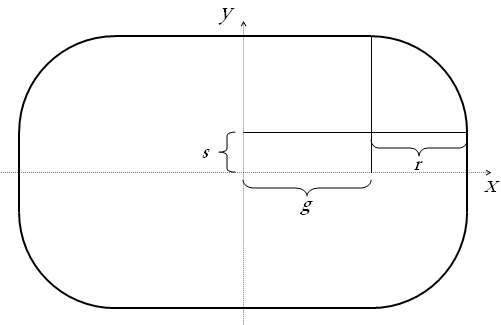
Syntax: APER_TOL = {r, g, s};

MB : SBEND, L := l.MB, APER_TOL={1.5, 1.1, 0};

APERTURE MODULE

Computes the n1 values for a piece of machine. Each element is sliced into thick subelements at given intervals, and the available aperture is computed at the end of each slice. The computation is based on the last Twiss table, so it is important to run the Twiss and aperture commands on the same period or sequence, see the aperture example below. Also showed in the example is how n1 values can be plotted.

The minimum n1 for each element is written to the last Twiss table, to allow for matching by aperture.

Aperture,
```
file=filename,
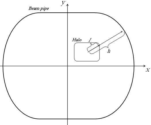
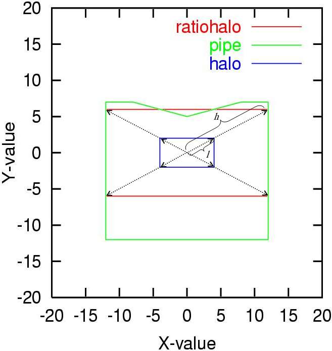
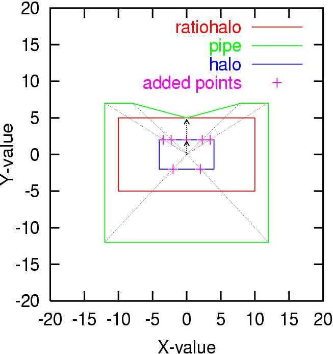
halofile=filename,
pipefile=filename,
range=range,
exn=real,
eyn=real,
dqf=real,
betaqfx=real,
dp=real,
dparx=real,
dpary=real,
cor=r,
bbeat=real,
nco=integer,
halo={real,real,real,real},
interval=real
spec=real,
notsimple=logical,
trueprofile=filename,
offsetelem=filename;
```
where the parameters have the following meaning:
- file: Output file with aperture table. Default = none
- halofile: Input file with halo polygon coordinates. Will suppress an eventual halo parameter. Default = none
- range: Range given by elements. Default = #s/#e
- exn: Normalised horizontal emittance. Default = 3.75*e-6
- eyn: Normalised vertical emittance. Default = 3.75*e-6
- dqf: Peak linear dispersion [m]. Default = 2.086
- betaqfx: Beta x in standard qf [m]. Default = 170.25
- dp: Bucket edge at the current beam energy. Default = 0.0015
- dparx: Fractional horizontal parasitic dispersion. Default = 0.273
- dpary: Fractional vertical parasitic dispersion. Default = 0.273
- cor: Maximum radial closed orbit uncertainty [m]. Default = 0.004
- bbeat: Beta beating coefficient applying to beam size. Default = 1.1
- nco: Number of azimuth for radial scan. Default = 5
- halo: Halo parameters: {n, r, h, v}. n is the radius of the primary halo, r is the radial part of the secondary halo, h and v is the horizontal and vertical cuts in the secondary halo. Default = {6, 8.4, 7.3, 7.3}
- interval: Approximate length in meters between measurements. Actual value: nslice = nodelength/interval, nslice is rounded down to closest integer, interval = nodelength/nslice. Default = 1.0
- spec: Aperture spec, for plotting only. Gives the spec line in the plot. Default = 0.0
- notsimple: Use only if one or more beamscreens in the range are considered not to be a "simply connex". Since all MAD-X apertypes are simply connex, this is only possible if an input file with beam screen coordinates are given. See below for a graphical example. Default = false.
- trueprofile: A file containing a list of magnets, and for each magnet a list of horizontal and vertical deviations from the ideal magnet axis. These values may come from measurements done on the magnet. See below for example. Default = none.
- offsetelem: A file containing a reference point in the machine, and a list of magnets with their offsets from this point described as a parabola. See below for example. Default = none.
Not simply connex beam pipes
Methodically, the algorithm for finding the largest possible halo is fairly simple. The distance from halo centre to the first apex (i = 0) in the halo is calculated (l_i), and the equation for a line going through these points is derived. This line is then compared with all lines making the pipe polygon to find their respective intersection coordinates. The distance h_i between halo centre and intersection are then divided by l_i, to find the maximal ratio of enlargement, as seen below. This procedure is then repeated for all apexes i in the halo polygon, and the smallest ratio of all apexes is the maximal enlargement ratio for this halo to just touch the pipe at this particular longitudinal position.

There is one complication to this solution; polygons which are not simple connexes. (Geometrical definition of ``simply connex'': A figure in which any two points can be connected by a line segment, with all points on the segment inside the figure.) The figure below shows what happens when a beam pipe polygon is not a simple connex. The halo is expanded in such a way that it overlaps the external polygon in the area where the latter is dented inwards.

To make the module able to treat all kinds of polygons, notsimple must be activated. With this option activated, apexes are strategically added to the halo polygon wherever the beam pipe polygon might have an inward dent. This is done by drawing a line from halo centre to each apex on the pipe polygon. An apex with its coordinates on the intersection point line-halo is added to a table of halo polygon apexes. The result is that the halo polygon has a few ``excessive'' points on straight sections, but the algorithm used for expansion will now never miss a dent in the beam pipe. The use of the notsimple option significantly increases computation time.

Trueprofile file syntax
This file contains magnet names, and their associated displacements of the axis for an arbitrary number of S, where So is the start of the magnet and Sn the end. The interval between each S must be regular, and X and Y must be given in meters. The magnet name must be identical to how it appears in the sequence. The displacements are only valid for this particular magnet, and cannot be assigned to a family of magnets. n1 is calculated for a number of slices determinated by the number of Si.

Layout of file:
```
magnet.name1
So   X   Y
Si   X   Y
Si   X   Y
Sn   X   Y

magnet.name2
So   X   Y
Si   X   Y
Si   X   Y
Sn   X   Y

etc.
```
Example of file:
```
!This is the start of the file.
!Comments are made with exclamation marks.

mb.a14r1.b1
0        0.0002        0.000004
7.15     1.4e-5        0.3e-3
14.3     0.0000000032  4e-6

!further comments can of course be added

mq.22r1.b1
0      0.3e-5     1.332e-4
1.033  0.00034    0.3e-9
2.066  0          0.00e-2
3.1    4.232e-4   0.00000003

!This is the end of the file.
```
Offsetelem file syntax
This file contains coordinates describing how certain elements are displaced w.r.t. a given reference point in the machine. It might be used with elements in insertions, or other special-purpose elements that has a magnet axis which does not coincide with the reference trajectory. We operate with two coordinate system, s,x and s,y, where the reference point is the origin and the actual element axis is described as a parabola with coefficients A, B and C. For each element we give two sets of coefficients, one for horizontal displacement and one for vertical:
```
X_offs(s) = Ax*s^2 + Bx*s + Cx 
```
and
```
Y_offs(s) = Ay*s^2 + By*s + Cy
```
. The coordinate systems are in meters.

Layout of file: --- FOR MADX VERSION 3.XX AND OLDER ONLY---
```
reference.point

magnet.name1
Ax   Bx   Cx
Ay   By   Cy

magnet.name2
Ax   Bx   Cx
Ay   By   Cy

etc.
```
Example of file:
```
!This is the start of the file.
!First we give a reference point. The origin of the 
!coordinate system will be at the START of this element.

mq.12r1.b1

!Then we give a list of elements and their displacement 
!w.r.t. the reference point.

mcbxa.3l2
0   -2.56545   -3
0   -2.3443666  0

!The next nodes use the same reference point.
!Elements offset w.r.t. another point must be given in another file,
!together with the new reference point.

mcbxa.3r2
0.3323  32.443355 -0.84
0.2522  32.554363 0.0

!This is the end of the file.
```
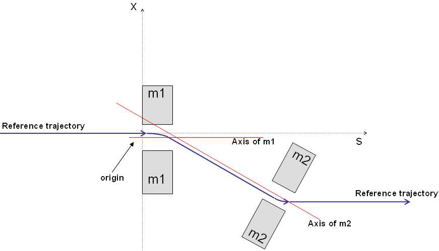
Layout of file: --- FOR MADX VERSION 4.XX ONWARDS : now TFS format ---
note that variable names changes with : Ax -> DDX_OFF, Bx -> DX_OFF, Cx -> X_OFF, same for Y The column S_IP is useless but mandatory (!). It results from a misunderstanding. Content is ignored. In a future version, it will be suppressed (but will not induce an error if present).
```
@ NAME             %06s "OFFSET" 
@ TYPE             %06s "OFFSET" 
@ REFERENCE        %10s "mq.12r1.b1" 
* NAME          S_IP       X_OFF     DX_OFF    DDX_OFF    Y_OFF    DY_OFF     DDY_OFF
"mq.12r1.b1"	0.0        -3.0      -2.56545    0.0       0.0    -2.3443666    0.0
"mcbxa.3r2"     0.0        -0.84     32.443355  0.3323     0.0    32.554363    0.2522

A python script to convert a file from the old V.3.XX format to the new V4.xx can be found at :

/afs/cern.ch/eng/lhc/optics/V6.503/aperture/convert_offsets.py

usage : convert_offsets.py filename
```
As an example we see in the picture below how the horizontal axes of elements m1 and m2 does not coincide with the reference trajectory.
The X_ref(s) and Y_ref(s) of the reference trajectory are calculated via an internal call to the Survey module. X_offs(s) and Y_offs(s) are derived from the coefficients given in the file. The resulting
```
X_tot(s) = X_ref(s) - X_offs(s)
```
and
```
Y_tot(s) = Y_ref(s) - Y_offs(s)
```
are taken into account in the aperture calculations.
Aperture command example

The aperture module needs a Twiss table to operate on. It is important not to USE another period or sequence between the Twiss and aperture module calls, else aperture looses its table. One can choose the ranges for Twiss and aperture freely, they need not be the same.
```
use, period=lhcb1;
select, flag=twiss,range=mb.a14r1.b1/mb.a17r1.b1,column=keyword,name,parent,k0l,k1l,s,betx,bety,n1;
twiss, file=twiss.b1.data, betx=beta.ip1, bety=beta.ip1, x=+x.ip1, y=+y.ip1, py=+py.ip1;
plot,haxis=s,vaxis=betx,bety,colour=100;

select, flag=aperture, column=name,n1,x,dy;
aperture, range=mb.b14r1.b1/mb.a17r1.b1, spec=5.235;
plot,table=aperture,noline,vmin=0,vmax=10,haxis=s,vaxis=n1,spec,on_elem,style=100;
```
The select command can be used to choose which columns to print in the output file.
Column names: name, n1, n1x_m, n1y_m, apertype, aper_1, aper_2, aper_3, aper_4, rtol, xtol, ytol, s, betx, bety, dx, dy, x, y, on_ap, on_elem, spec
n1 is the maximum beam size in sigma, while n1x_m and n1y_m is the n1 values in si-units in the x- and y-direction.
aper_# means for all apertypes but racetrack:
aper_1 = half width rectangle
aper_2 = half heigth rectangle
aper_3 = half horizontal axis ellipse (or radius if circle)
aper_4 = half vertical axis ellipse
For racetrack, the aperture parameters will have the same meaning as the tolerances:
aper_1 and xtol = horizontal displacement of radial part
aper_2 and ytol = vertical displacement of radial part
aper_3 and rtol = radius
aper_4 = not used
On_elem indicates whether the node is an element or a drift, and on_ap whether it has a valid aperture. The Twiss parameters are the interpolated values used for aperture computation.
When one wants to plot the aperture, the table=aperture parameter is necessary. The normal line of hardware symbols along the top is not compatible with the aperture table, so it is best to include noline. Plot instead the column on_elem along the vaxis to have a simple picture of the hardware. Spec can be used for giving a limit value for n1, to have something to compare with on the plot. This example provides a plot,

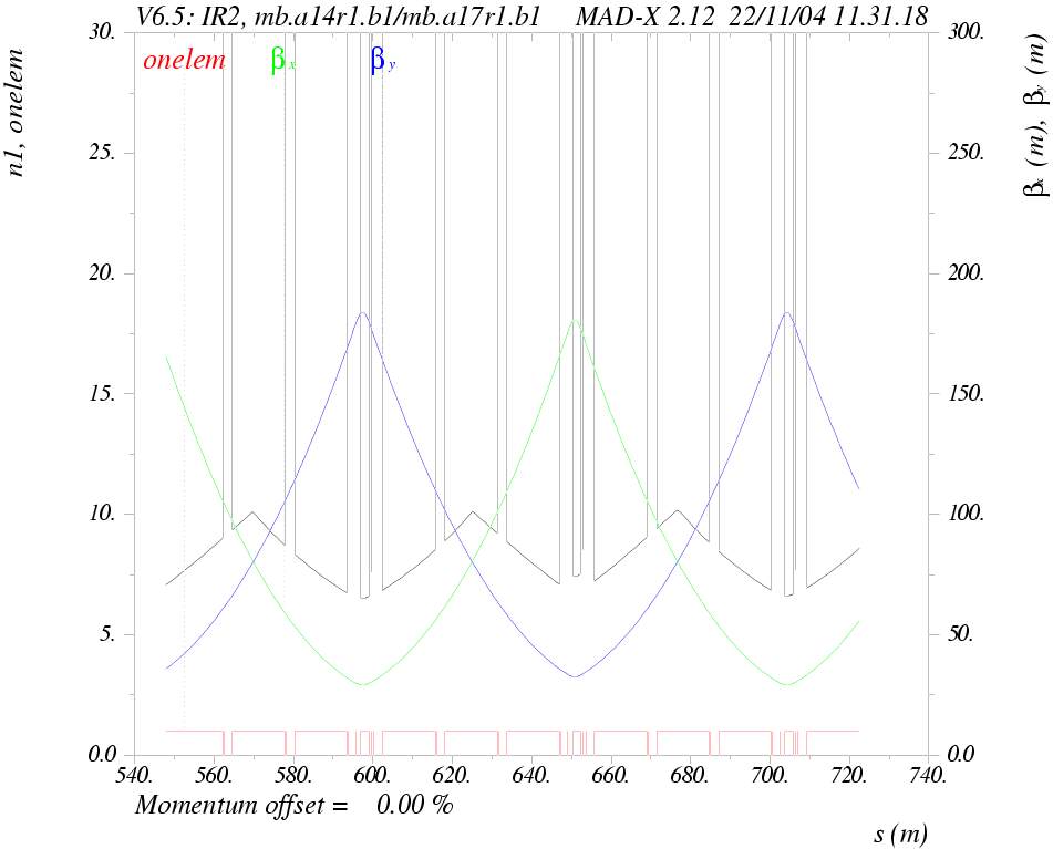
where we see the n1, beta functions and the hardware symbolized by on_elem.

Ivar Waarum, 24.02.05 - Mark Hayes, 19.06.02

Defining aperture in MAD-X

Defining tolerances in MAD-X

APERTURE MODULE

Aperture,

Not simply connex beam pipes

Trueprofile file syntax

Layout of file:

Example of file:

Offsetelem file syntax

Layout of file: --- FOR MADX VERSION 3.XX AND OLDER ONLY---

Example of file:

Layout of file: --- FOR MADX VERSION 4.XX ONWARDS : now TFS format ---

Aperture command example